The Syrup Basics
Properties of the Universal Gate nand
We are given a big pile of
nand
gates and have to build everything in terms of them. First things
first, we can check the
type of
nand (syrup tells us it takes
two bits as inputs and produces one bit as output) as well as
experiment with it (we get the expected
truth table).
|
Typing for nand:
nand(<Bit>, <Bit>) -> <Bit>
Truth table for nand:
X Y |
----|--
0 0 | 1
0 1 | 1
1 0 | 1
1 1 | 0 |
Our First Definition: the not Gate
Using the universal gate
nand,
we can build the
not gate:
- The first line is a type declaration: we introduce a gate named
not and state that it takes one
input and returns one output (both of type <Bit>).
- The second line is the gate's definition: we name its one input
X, duplicate it, feed both
Xs to
nand and immediately return
the result.
Feel free to
experiment with the
newly created gate.
Reusing Definitions: Building and and or
By applying the same principles, we can build the other fundamental
logic gates
and and
or using their standard implementation
in terms of
nand and
not (note that we have syntactic sugar:
prefix
! for
not).
Displaying Circuits
Running an
experiment can help us
convince ourselves that we have indeed defined the gates we meant to
define. But for bigger circuits, it will get rather fastidious to
check every single line of a truth table.
If we already have a hand-drawn diagrammatic solution, we can check
that the code we have written corresponds to a circuit that has the
same structure by using
display
to automatically render our code.
Feel free to render other circuits. Note that you can unfold
subcircuits such as
not by using
the syntax
display
[not]
and
where the list in the middle is a comma-separated list of circuit
names (
nand is a primitive and, as
such, cannot be unfolded).
Our worked example: rca3
In the paper we explain how, assuming that we know the basics of
addition, we can build a riple-carry adder for 3 bit inputs.
The basics of addition
In order to build complex arithmetic circuits, we assume that we
have already defined
exclusive or (
xor),
a half adder taking two bits and returning two bits representing their sum
(
hadd),
and a full adder taking two bits and a carry-in and returning a bit and a carry-out
representing the total sum (
fadd).
You can in fact inspect all of these definitions by using
print.
You will notice a few things:
- We have syntactic sugar for and
(infix &)
and or
(infix |)
- For circuits with multiple outputs (e.g. hadd),
we simply list the expressions computing each of the outputs
using commas as separators
- For circuits relying on intermediate results, we can use a
where clause to explain how
these intermediate signals are computed. This clause is made out
of equations with, on the left-hand side, a list of names for each
of the computed outputs, and, on the right-hand side, the expression
producing these outputs.
|
Printing xor:
xor(<Bit>, <Bit>) -> <Bit>
xor(X, Y) = X & !Y | !X & Y
Printing hadd:
hadd(<Bit>, <Bit>) -> <Bit>, <Bit>
hadd(X, Y) = X & Y, xor(X, Y)
Printing fadd:
fadd( <Bit>, <Bit>, <Bit>) -> <Bit>, <Bit>
fadd( X, Y, Cin) = Cout, Z where
A2, A1 = hadd(X, Y)
B2, Z = hadd(A1, Cin)
Cout = A2 | B2 |
Feel free to, once again, use
experiment to access the
circuits' truth tables, or
display
to inspect the diagrams these definitions induce.
RCA3 from a diagram
Let us say that we have produced the following diagram by working
through the problem of adding two 3 bit numbers and a carry-in
by repeatedly using
fadds to add digits of the same
place value, adding type information at the circuit's interface, and
naming the outputs as well as the intermediate results (the various
carry forwards).
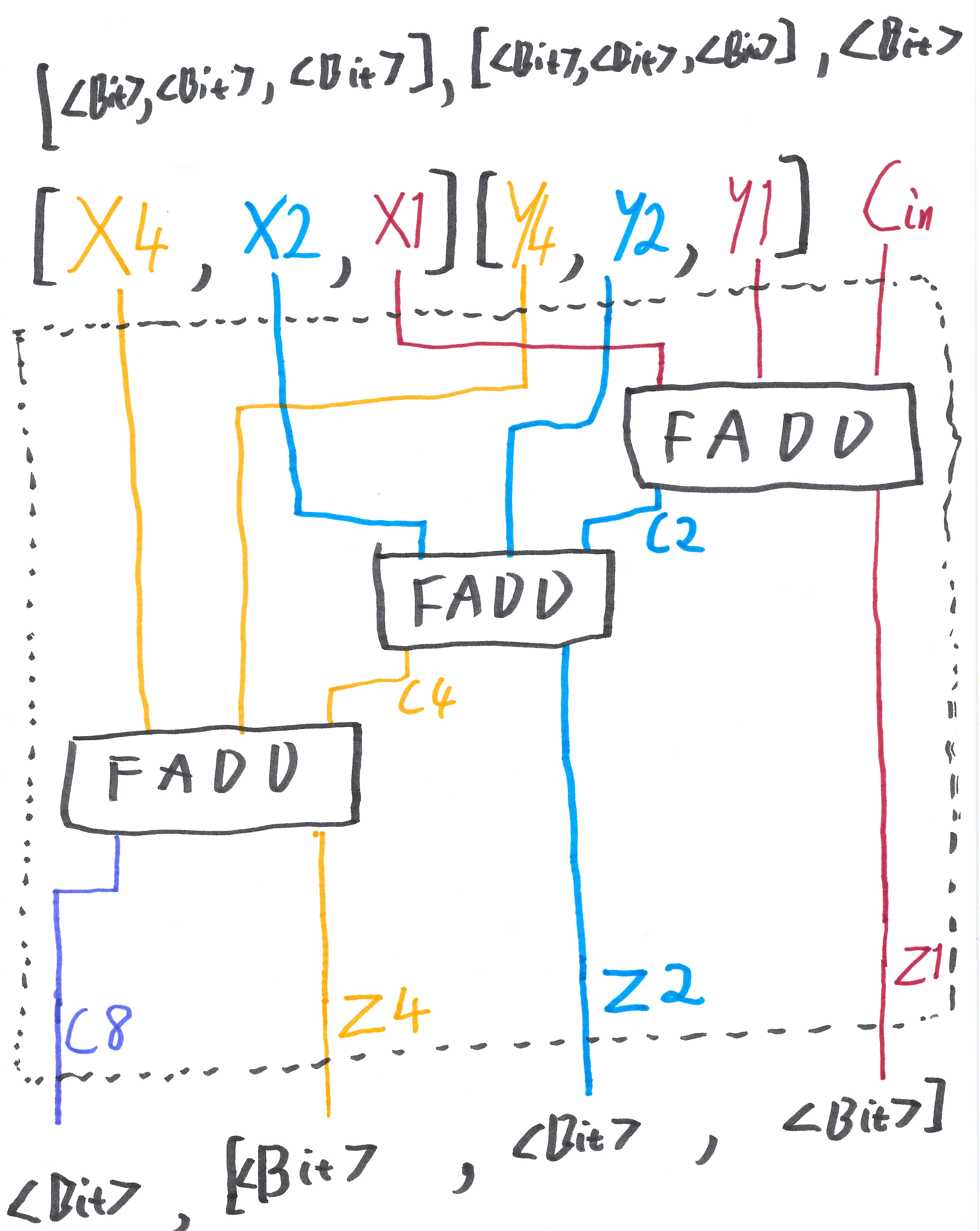
We can read off the syrup code by
- Introducing a type alias
<Bit3> for
cables of 3 bits to avoid repeating ourselves
in the types
- Declaring the circuit rca3
that takes two cables of 3 bits and a carry-in
- Starting to define rca3
by splitting the input cables open using cable patterns
(e.g. [X4,
X2,
X1])
and describing the output as a cable packing 3 bits together.
- Building a where clause
listing the intermediate computations that give a meaning to
the signals used in the output but not yet defined.
You can close the DED loop by rendering the diagram for rca3 in order
to check that it indeed has the same overall structure as our handwritten
solution. We did not make a mistake when encoding the circuit in Syrup!
Circuit Equivalences
Visualising circuits is useful beyond just checking our work.
We will see below how we can use
display
to spot simplification opportunities, and then rely on
experiment
to ensure that our simplified circuits still have the same behaviour.
Fearless refactoring!
Inlining hadds
in fadd
Looking at the rendered
fadd
with
hadd unfolded, we can start
spotting simplification opportunities.
For instance, the output
Cout
is computed as the
or of
two
ands.
But
or is just
nand with both of its inputs
negated, and
and is
nand with its ouput negated.
Therefore the
or of
two
ands has two needless
double negations.
We can make this more explicit by rewriting
fadd with the
hadds inlined
and this
Cout
computation simplified.
Using the
cost
experiment we can verify that
fadd2 is indeed
cheaper than
fadd.
But are they equivalent? We can check this using an
equality experiment!
|
Displaying fadd (with hadd unfolded):
Cost for fadd:
25 copies of nand
Cost for fadd2:
21 copies of nand
Bisimulation between fadd, fadd2:
fadd behaves like fadd2
{} ~ {}
|
Simplifying xor
We can observe exactly the same pattern in the definition of
xor: it is a disjunction
of conjunctions and can therefore be simplified.
Using this updated definition to implement an even further
optimised
fadd3 gives
us a final adder that's half as expensive as the original one!
|
Printing xor:
xor(<Bit>, <Bit>) -> <Bit>
xor(X, Y) = X & !Y | !X & Y
Cost for xor:
9 copies of nand
Cost for xor2:
5 copies of nand
Bisimulation between xor, xor2:
xor behaves like xor2
{} ~ {}
Cost for fadd:
25 copies of nand
Cost for fadd3:
13 copies of nand
Bisimulation between fadd, fadd3:
fadd behaves like fadd3
{} ~ {}
|